# Optimizing AlphaFold's Triangle Multiplicative Update: A First Look at GPU Performance Engineering

URL: https://www.msuiche.com/posts/optimizing-alphafolds-triangle-multiplicative-update-a-first-look-at-gpu-performance-engineering/
Date: 2025-09-30
Author: Matt Suiche
Tags: GPU Optimization, PyTorch, Triton, AlphaFold, Machine Learning, Performance Engineering, H100, Tensor Cores


> Learning GPU performance engineering through the GPU MODE TriMul challenge - achieving 2.42× speedup on H100 through FP16 optimization, weight fusion, and systematic experimentation.

---


## Background

I recently encountered the [GPU MODE TriMul challenge](https://www.gpumode.com/v2/leaderboard/496?tab=submission) while exploring GPU optimization. Coming from a systems engineering background without prior PyTorch or Triton experience, this challenge provided an opportunity to learn GPU performance engineering through a practical problem.

The Triangle Multiplicative Update (TriMul) is a core operation in AlphaFold2 and AlphaFold3—the protein structure prediction systems that earned the 2024 Nobel Prize in Chemistry. The operation's O(n³) complexity creates severe performance bottlenecks in production, forcing AlphaFold3 to use batch size 1 during training despite having under 1B parameters. This makes the optimization problem both practically relevant and technically challenging.

GPU MODE's educational content, particularly their technical deep-dives, proved invaluable while learning these concepts. Their focus on real-world problems rather than toy examples made the learning process significantly more effective.

Stay with me, this blogpost is quite lengthy as I've literally been brain dumping a lot of things I've seen and learned over the past months. 

## Problem Definition

### Mathematical Formulation

The TriMul operation computes pairwise interactions in protein structure prediction:

```python
# Critical O(n³) einsum
out = einsum('bikh,bjkh->bijh', left, right)

# Equivalent to nested loops:
for b in range(batch_size):
    for i in range(seq_len):
        for j in range(seq_len):
            for k in range(seq_len):
                for h in range(hidden_dim):
                    out[b,i,j,h] += left[b,i,k,h] * right[b,j,k,h]
```

**Complexity**: O(B × N³ × H) where:
- B = batch size
- N = sequence length
- H = hidden dimension

For N=1024, H=128: approximately 134 billion floating point operations per batch.

### Performance Target

**H100 Leaderboard (at project start):**

| Rank | Submitter | Time | Delta from #1 |
|------|-----------|------|---------------|
| 1st | davidberard | 1.371ms | - |
| 2nd | Waqar | 2.368ms | +996μs |
| 3rd | [Arseni Ivanov](https://arseniivanov.github.io/blog.html) | 2.546ms | +178μs |
| 4th | Apeirogon | 3.655ms | +1109μs |

**My Results:**

| Implementation               | Time (geometric mean) | vs Baseline   | Status                  |
|------------------------------|-----------------------|---------------|-------------------------|
| Reference baseline           | 10.154ms              | 1.00×         | Starting point          |
| submission_improved_triton.py| **2.399ms**           | 4.23× faster  | [See at the end of the blogpost](#three-way-hybrid-implementation) |
| **PyTorch optimized**        | **4.201ms**           | **2.42× faster** | ⚡ Best               |
| CUDA naive                   | 35.107ms              | 0.29× slower  | 🐌 Significantly slower |


**Target:** Sub-3ms for top-3 leaderboard placement (not achieved).

## Development Environment: Modal.com Integration

Testing on actual H100 hardware without repeatedly submitting to gpumode required a cloud GPU solution. I implemented a Modal.com-based testing harness that enabled rapid iteration on both PyTorch and CUDA implementations.

### Why Modal?

**Problem:** Need H100 access for:
- Testing PyTorch/Triton optimizations
- Compiling and benchmarking CUDA kernels
- Rapid iteration without expensive hardware (I have none)

**Solution:** Modal provides:
- On-demand H100 access ($3-4/hour)
- Fast cold starts (~10 seconds)
- Python-native API
- Automatic dependency management

### Implementation

Modal is a serverless platform for GPU workloads. (_Here is a good presentation to look for about isolation for GPU Cloud architecture: [chompie & Sam's presentation](https://www.hexacon.fr/conference/speakers/#cuda_de_grace)_) The integration mirrors gpumode's evaluation environment:

```python
import modal

app = modal.App(name="trimul-gpu-benchmark")

# For CUDA development: Use NVIDIA CUDA development image
gpu_image = modal.Image.from_registry(
    "nvidia/cuda:12.4.0-devel-ubuntu22.04",  # Includes nvcc, CUDA headers
    add_python="3.11"
).apt_install(
    "build-essential"  # GCC, g++, make for compilation
).pip_install(
    "torch", "triton", "pyyaml", "numpy",
    "ninja"  # Required for PyTorch JIT compilation
)

@app.function(image=gpu_image, gpu="H100", timeout=1800)
def run_remote_benchmark(mode, task_file_content, sources, verbose=False):
    """Execute benchmarks on Modal's H100 infrastructure."""
    import os
    import tempfile
    from pathlib import Path

    # Set CUDA environment for JIT compilation
    os.environ['CUDA_HOME'] = '/usr/local/cuda'
    os.environ['TORCH_CUDA_ARCH_LIST'] = '9.0'  # H100 = sm_90

    with tempfile.TemporaryDirectory() as tmpdir:
        os.chdir(tmpdir)

        # Write all source files (Python + CUDA + C++)
        for filename, content in sources.items():
            Path(filename).write_text(content)

        # Execute evaluation
        from run_eval import run_config
        result = run_config(config)

        return result
```

**Key configuration for CUDA:**
- Use `-devel` image (not just runtime)
- Install `ninja` for PyTorch JIT
- Set `CUDA_HOME` environment variable
- Include all source files in upload (`.cu`, `.cpp`, `.py`)

### Usage

```bash
# Install and authenticate Modal CLI
pip install modal
modal setup

# Run benchmarks on H100
MODAL_MODE=benchmark modal run run_modal.py

# Run correctness tests only
MODAL_MODE=test modal run run_modal.py

# Check GPU availability
MODAL_CHECK_GPU=true modal run run_modal.py
```

### Internal Operation

1. **Local phase**: Script reads `submission.py`, `task.yml`, and all source files (`.cu`, `.cpp`, `.py`)
2. **Image build** (first run only): Modal builds Docker image with CUDA toolkit (~2 minutes)
3. **Upload**: Source files transferred to Modal infrastructure via `.remote()` call
4. **Provisioning**: Modal allocates H100 GPU instance (<10 seconds cold start)
5. **CUDA compilation**: PyTorch JIT compiles `.cu` files with `nvcc` (~30-60 seconds)
6. **Execution**: Benchmarks run with compiled CUDA kernel
7. **Results**: Performance metrics stream back in real-time
8. **Cleanup**: Container and GPU automatically destroyed

**Iteration speed:**
- First run: ~3-4 minutes (image build + compilation)
- Subsequent runs: ~1-2 minutes (cached image, recompilation only)
- Image cached for 7 days

This workflow enabled rapid CUDA kernel development without owning H100 hardware or waiting in submission queues.

## Final PyTorch Implementation: submission.py (4.201ms)

After testing multiple approaches including CUDA implementations, the best-performing implementation achieved **4.201ms geometric mean** - a **2.42× speedup** over the reference H100 baseline of 10.154ms. This pure PyTorch implementation significantly outperformed hand-written CUDA (35.107ms).

### Optimization Strategy

The optimization approach follows a hierarchical strategy targeting different performance bottlenecks:

```mermaid
graph TD
    A[Reference Implementation<br/>10.154ms] --> B[Strategy 1: Weight Fusion<br/>~1.3× speedup]
    B --> C[Strategy 2: FP16 Pipeline<br/>~1.4× speedup]
    C --> D[Strategy 3: BMM over Einsum<br/>~1.2× speedup]
    D --> E[Strategy 4: Memory Contiguity<br/>~1.1× speedup]
    E --> F[Strategy 5: Backend Flags<br/>~1.05× speedup]
    F --> G[Optimized Implementation<br/>4.201ms = 2.42× total]

    style A fill:#ffcccc
    style G fill:#ccffcc
    style B fill:#fff4cc
    style C fill:#fff4cc
    style D fill:#fff4cc
    style E fill:#fff4cc
    style F fill:#fff4cc
```

**Key Optimizations:**

1. **FP16 pipeline**: Maximize H100 Tensor Core utilization
2. **Weight fusion**: Single 5H×D matmul instead of five H×D matmuls
3. **BMM over einsum**: Better memory access patterns for cuBLAS
4. **Memory contiguity**: Explicit `.contiguous()` before critical operations
5. **Backend flags**: Enable all available H100 optimizations

These optimizations are **multiplicative**: 1.3 × 1.4 × 1.2 × 1.1 × 1.05 ≈ 2.42×

### ⚠️ Warning: `.contiguous()` Performance Tradeoffs

While `.contiguous()` is necessary for optimal cuBLAS performance, it comes with costs:

**When it helps:**
- Before `torch.bmm()` or `torch.matmul()` with cuBLAS
- Enables optimal memory access patterns for Tensor Cores
- In this case: **essential** for 4ms performance

**When it hurts:**
- Creates full memory copies (expensive for large tensors)
- Can be 2x+ slower than layout-aware approaches
- Generic operation that doesn't optimize for specific access patterns

As detailed in my [Gluon deep-dive](https://www.msuiche.com/posts/gluon-when-triton-isnt-low-level-enough/), specialized layout conversions (like Gluon's transpose tricks) can achieve >2x better bandwidth than generic `.contiguous()`. However, without low-level control, I'm stuck with PyTorch's generic path.

**In this implementation:** The contiguity overhead is worth it because cuBLAS gains outweigh the copy cost. For larger tensors or different access patterns, this tradeoff might reverse.

### Core Implementation

The implementation follows a carefully optimized pipeline, with each step contributing to the overall 2.42× speedup:

```python
def _custom_kernel_core(data: input_t) -> output_t:
    input_tensor, mask, weights, config = data
    B, N, _, D = input_tensor.shape
    H = config["hidden_dim"]
    M = B * N * N

    # LayerNorm in FP32 (required for numerical stability)
    x = F.layer_norm(
        input_tensor, (D,),
        weight=weights["norm.weight"],
        bias=weights["norm.bias"],
        eps=1e-5
    )

    # Fuse 5 projection matrices into single matmul
    W_key = "__W_h16__"
    if W_key not in weights:
        weights[W_key] = torch.cat([
            weights['left_proj.weight'],
            weights['right_proj.weight'],
            weights['left_gate.weight'],
            weights['right_gate.weight'],
            weights['out_gate.weight'],
        ], dim=0).half()

    # Single fused projection (FP16)
    x_T = x.view(M, D).t().half()
    P = torch.matmul(weights[W_key], x_T).view(5, H, M)

    # Gating operations (FP16)
    LEFT_T = torch.sigmoid(P[2]) * P[0]
    if mask.min() < 1.0:
        LEFT_T *= mask.view(1, M).half()
    RIGHT_T = torch.sigmoid(P[3]) * P[1]
    OG_T = torch.sigmoid(P[4])

    # Prepare for BMM with contiguous memory layout
    LEFT_bhnn = LEFT_T.view(H, B, N, N).permute(1, 0, 2, 3).contiguous()
    RIGHT_bhnn = RIGHT_T.view(H, B, N, N).permute(1, 0, 2, 3).contiguous()

    LEFT_flat = LEFT_bhnn.view(B * H, N, N)
    RIGHT_flat = RIGHT_bhnn.view(B * H, N, N)

    # Critical einsum rewritten as BMM
    # einsum('bikh,bjkh->bijh') becomes bmm
    EIN_flat = torch.bmm(LEFT_flat, RIGHT_flat.transpose(1, 2))

    # Reshape output
    EIN = EIN_flat.view(B, H, N, N).permute(0, 2, 3, 1).contiguous()

    # Output processing
    OG = OG_T.view(H, B, N, N).permute(1, 2, 3, 0)
    G = F.layer_norm(
        EIN.float(), (H,),
        weight=weights['to_out_norm.weight'],
        bias=weights['to_out_norm.bias'],
        eps=1e-5
    ) * OG.float()

    # Final projection
    Wt_key = "__Wt_h16__"
    if Wt_key not in weights:
        weights[Wt_key] = weights['to_out.weight'].t().half()

    OUT = torch.matmul(G.half().view(M, H), weights[Wt_key]).float()
    return OUT.view(B, N, N, D)
```

#### Step-by-Step Breakdown

**1. Input LayerNorm (FP32)**

```python
x = F.layer_norm(input_tensor, (D,), weight=weights["norm.weight"],
                 bias=weights["norm.bias"], eps=1e-5)
```

- Keeps FP32 precision for numerical stability
- LayerNorm requires accurate statistics computation
- This step has minimal performance impact (~5% of total time)

**2. Weight Fusion (~1.3× speedup)**

Weight fusion consolidates multiple projection matrices into a single matrix multiplication, reducing kernel launch overhead:

```mermaid
graph LR
    subgraph "Before: 5 Separate Matmuls"
        X1[Input X<br/>M×D] --> LP[left_proj<br/>H×D]
        X1 --> RP[right_proj<br/>H×D]
        X1 --> LG[left_gate<br/>H×D]
        X1 --> RG[right_gate<br/>H×D]
        X1 --> OG[out_gate<br/>H×D]
        LP --> O1[5 separate<br/>GPU kernels]
        RP --> O1
        LG --> O1
        RG --> O1
        OG --> O1
    end

    subgraph "After: 1 Fused Matmul"
        X2[Input X<br/>M×D] --> W[Fused Weight<br/>5H×D]
        W --> O2[1 GPU kernel<br/>~1.3× faster]
    end

    style O1 fill:#ffcccc
    style O2 fill:#ccffcc
```

**Implementation:**

```python
W_key = "__W_h16__"
if W_key not in weights:
    weights[W_key] = torch.cat([
        weights['left_proj.weight'],
        weights['right_proj.weight'],
        weights['left_gate.weight'],
        weights['right_gate.weight'],
        weights['out_gate.weight'],
    ], dim=0).half()  # [5H, D] in FP16
```

**Benefits:**
- Concatenates 5 separate weight matrices into a single [5H, D] matrix
- Converts to FP16 once and caches the result
- **Key optimization**: Replaces 5 separate matmuls with 1 large matmul
- Reduces kernel launch overhead (5 launches → 1 launch)
- Improves memory locality (better cache utilization)

**3. Single Fused Projection (~1.4× speedup from FP16)**

FP16 precision enables Tensor Core acceleration on H100, delivering ~2× throughput compared to FP32:

```mermaid
graph TD
    subgraph "FP32 Path (Slow)"
        I1[Input FP32<br/>M×D] --> TC1{Tensor Cores?}
        TC1 -->|Not used| ALU1[ALU Units<br/>FP32 FFMA]
        ALU1 --> R1[Result<br/>~2× slower]
    end

    subgraph "FP16 Path (Fast)"
        I2[Input FP16<br/>M×D] --> W2[Fused Weight FP16<br/>5H×D]
        W2 --> TC2[Tensor Cores<br/>FP16 GEMM]
        TC2 --> R2[Result 5H×M<br/>~1.4× faster]
    end

    style R1 fill:#ffcccc
    style R2 fill:#ccffcc
    style TC2 fill:#cceeff
```

**Implementation:**

```python
x_T = x.view(M, D).t().half()  # Convert to FP16
P = torch.matmul(weights[W_key], x_T).view(5, H, M)
```

**Benefits:**
- Converts input to FP16 for Tensor Core utilization
- Single matmul: [5H, D] × [D, M] → [5H, M]
- H100 Tensor Cores deliver 2× throughput for FP16 vs FP32
- Result contains all 5 projections stacked together

**4. Gating Operations (FP16)**

```python
LEFT_T = torch.sigmoid(P[2]) * P[0]
if mask.min() < 1.0:
    LEFT_T *= mask.view(1, M).half()
RIGHT_T = torch.sigmoid(P[3]) * P[1]
OG_T = torch.sigmoid(P[4])
```

- Applies gated linear units (GLU) to projections
- All operations in FP16 for consistency
- Mask application fused with gating when needed

**5. BMM over Einsum (~1.2× speedup)**

```python
LEFT_bhnn = LEFT_T.view(H, B, N, N).permute(1, 0, 2, 3).contiguous()
RIGHT_bhnn = RIGHT_T.view(H, B, N, N).permute(1, 0, 2, 3).contiguous()

LEFT_flat = LEFT_bhnn.view(B * H, N, N)
RIGHT_flat = RIGHT_bhnn.view(B * H, N, N)

EIN_flat = torch.bmm(LEFT_flat, RIGHT_flat.transpose(1, 2))
```

**What is BMM?**

BMM stands for **Batch Matrix Multiply** - a specialized operation that performs many independent matrix multiplications in parallel:

```python
# BMM: Given two 3D tensors [batch, m, k] and [batch, k, n]
# Performs: output[i] = A[i] @ B[i] for each i in batch
# Result: [batch, m, n]

# Example:
A = torch.randn(100, 64, 32)  # 100 matrices of size 64×32
B = torch.randn(100, 32, 128) # 100 matrices of size 32×128
C = torch.bmm(A, B)            # 100 matrices of size 64×128
```

**BMM vs Einsum**

The original operation uses einsum notation:
```python
# Einsum: flexible but generic
einsum('bikh,bjkh->bijh', left, right)
# Meaning: for each (b,i,j,h), sum over k: left[b,i,k,h] * right[b,j,k,h]
```

I rewrote it as BMM:
```python
# BMM: specialized for matrix multiplication
# Reshape to [B*H, N, N] to treat each (batch, hidden) pair as independent
bmm(LEFT_flat, RIGHT_flat.transpose(1, 2))
```

```mermaid
graph TD
    subgraph "Einsum Path (Generic)"
        E1[einsum'bikh,bjkh->bijh'] --> E2[Parse subscripts<br/>at runtime]
        E2 --> E3[Analyze pattern]
        E3 --> E4[Dispatch to<br/>generic kernel]
        E4 --> E5[Result<br/>slower]
    end

    subgraph "BMM Path (Optimized)"
        B1[Reshape to<br/>B*H, N, N] --> B2[torch.bmm]
        B2 --> B3[Direct cuBLAS<br/>GEMM call]
        B3 --> B4[Tensor Core<br/>optimized]
        B4 --> B5[Result<br/>~1.2× faster]
    end

    style E5 fill:#ffcccc
    style B5 fill:#ccffcc
    style B3 fill:#cceeff
    style B4 fill:#cceeff
```

**Why BMM is faster:**

1. **Specialized CUDA kernels**: cuBLAS provides highly optimized GEMM kernels specifically for BMM
2. **Direct hardware mapping**: BMM maps directly to Tensor Core operations without intermediate conversions
3. **Better memory patterns**: Contiguous matrix layouts enable coalesced memory access
4. **Less dispatch overhead**: Einsum must analyze the subscript pattern at runtime; BMM goes straight to optimized code path

**The transformation:**

```python
# Original: einsum('bikh,bjkh->bijh')
# This computes: out[b,i,j,h] = Σ_k left[b,i,k,h] * right[b,j,k,h]

# Rewritten as BMM:
# 1. Reshape: [B, H, N, N] → [B*H, N, N] (treat B*H as batch dimension)
# 2. Transpose right: [B*H, N, N] → [B*H, N, N].transpose(1,2)
# 3. BMM: [B*H, N, N] @ [B*H, N, N] → [B*H, N, N]
# 4. Reshape back: [B*H, N, N] → [B, H, N, N] → [B, N, N, H]
```

**Performance impact**: This seemingly simple change gives ~1.2× speedup because:
- Einsum is a general-purpose operation that supports arbitrary tensor contractions
- BMM is a specialized fast path that directly calls highly optimized cuBLAS GEMM kernels
- **Key optimization**: `.contiguous()` ensures optimal cuBLAS performance by guaranteeing memory layout

**6. Reshape Output (~1.1× speedup from memory contiguity)**

Memory contiguity ensures optimal access patterns for subsequent operations:

```mermaid
graph LR
    subgraph "Non-Contiguous (Slow)"
        T1[Tensor<br/>strided layout] --> M1[Memory reads<br/>scattered]
        M1 --> C1[Cache misses]
        C1 --> R1[Result<br/>slower]
    end

    subgraph "Contiguous (Fast)"
        T2[Tensor<br/>contiguous] --> M2[Memory reads<br/>sequential]
        M2 --> C2[Cache hits]
        C2 --> R2[Result<br/>~1.1× faster]
    end

    style R1 fill:#ffcccc
    style R2 fill:#ccffcc
    style C2 fill:#cceeff
```

**Implementation:**

```python
EIN = EIN_flat.view(B, H, N, N).permute(0, 2, 3, 1).contiguous()
```

**Benefits:**
- Reshapes BMM output to expected dimensions
- `.contiguous()` ensures sequential memory layout
- Enables coalesced memory access for downstream operations
- Critical for optimal cuBLAS performance

**7. Output Processing**

```python
OG = OG_T.view(H, B, N, N).permute(1, 2, 3, 0)
G = F.layer_norm(
    EIN.float(), (H,),
    weight=weights['to_out_norm.weight'],
    bias=weights['to_out_norm.bias'],
    eps=1e-5
) * OG.float()
```

- Output LayerNorm in FP32 for numerical stability
- Multiplies by output gate
- Converting to FP32 here is required for accurate statistics

**8. Final Projection**

```python
Wt_key = "__Wt_h16__"
if W_key not in weights:
    weights[Wt_key] = weights['to_out.weight'].t().half()

OUT = torch.matmul(G.half().view(M, H), weights[Wt_key]).float()
return OUT.view(B, N, N, D)
```

- Projects from hidden dimension H back to input dimension D
- Uses cached transposed FP16 weights
- Final conversion to FP32 for output

#### What Contributed to the 2.42× Speedup

Breaking down the improvement from H100 baseline (10.154ms) to optimized submission (4.201ms):

1. **Weight Fusion** (~1.3×): Single 5H×D matmul instead of five separate H×D operations
2. **FP16 Pipeline** (~1.4×): Consistent half-precision for Tensor Core utilization
3. **BMM over Einsum** (~1.2×): Better cuBLAS kernel mapping and memory patterns
4. **Memory Contiguity** (~1.1×): Explicit `.contiguous()` before critical operations
5. **Backend Flags** (~1.05×): Optimal cuDNN/TF32 configuration (see Backend Configuration)

**Combined effect**: 1.3 × 1.4 × 1.2 × 1.1 × 1.05 ≈ 2.42×

These optimizations are multiplicative because they target different bottlenecks: weight fusion reduces kernel launches, FP16 increases compute throughput, BMM improves memory access, and contiguity ensures optimal cuBLAS performance.

### Backend Configuration

Backend flags provide the final ~1.05× speedup by enabling H100-specific optimizations. Each flag targets different hardware features:

```python
def custom_kernel(data: input_t) -> output_t:
    with DisableCuDNNTF32():  # Constraint from challenge
        # Enable matmul TF32 (separate from cuDNN TF32)
        torch.backends.cuda.matmul.allow_tf32 = True
        torch.set_float32_matmul_precision('high')

        # Enable reduced precision reductions
        if hasattr(torch.backends.cuda.matmul, 'allow_bf16_reduced_precision_reduction'):
            torch.backends.cuda.matmul.allow_bf16_reduced_precision_reduction = True
        if hasattr(torch.backends.cuda.matmul, 'allow_fp16_reduced_precision_reduction'):
            torch.backends.cuda.matmul.allow_fp16_reduced_precision_reduction = True

        # Enable optimized attention kernels
        if hasattr(torch.backends.cuda, 'enable_flash_sdp'):
            torch.backends.cuda.enable_flash_sdp(True)
        if hasattr(torch.backends.cuda, 'enable_mem_efficient_sdp'):
            torch.backends.cuda.enable_mem_efficient_sdp(True)
        if hasattr(torch.backends.cuda, 'enable_math_sdp'):
            torch.backends.cuda.enable_math_sdp(True)

        # Enable cuDNN autotuning
        torch.backends.cudnn.benchmark = True

        return _custom_kernel_core(data)
```

#### Backend Flags Explained

| Flag | Purpose | Impact | Why It Matters |
|------|---------|--------|----------------|
| **`torch.backends.cuda.matmul.allow_tf32`** | Enables TensorFloat-32 for matmul operations | ~1.3× faster FP32 matmul on Ampere/Hopper | Uses Tensor Cores for FP32 operations with FP32 range but reduced mantissa (19-bit → 10-bit). Separate from cuDNN TF32. |
| **`torch.set_float32_matmul_precision('high')`** | Sets global matmul precision mode | Confirms TF32 usage | Alternative way to enable TF32. Options: 'highest' (FP32), 'high' (TF32), 'medium' (BF16). |
| **`allow_bf16_reduced_precision_reduction`** | Allows BF16 accumulation in reductions | Faster sum/mean operations | Reduces precision in reduction loops (sum, mean) from FP32 to BF16 accumulation. Trade accuracy for speed. |
| **`allow_fp16_reduced_precision_reduction`** | Allows FP16 accumulation in reductions | Faster sum/mean operations | Similar to BF16 but uses FP16. More aggressive accuracy tradeoff. Critical for the FP16 pipeline. |
| **`enable_flash_sdp`** | Enables Flash Attention for scaled dot-product | Memory-efficient attention | Not directly used here, but enables Flash Attention if attention layers exist. No overhead if unused. |
| **`enable_mem_efficient_sdp`** | Enables memory-efficient attention | Lower memory usage | Alternative attention implementation. No overhead if unused. |
| **`enable_math_sdp`** | Enables standard math attention | Fallback for attention | Standard attention path. No overhead if unused. |
| **`torch.backends.cudnn.benchmark`** | Enables cuDNN autotuning | 1-5% speedup after warmup | Benchmarks multiple cuDNN algorithms at first run, caches best choice. Essential for production workloads with fixed input shapes. |

#### Key Insights

**TF32 vs FP32:**
- TF32 maintains FP32 range (8-bit exponent) but reduces mantissa from 23 bits to 10 bits
- On H100: TF32 uses Tensor Cores, FP32 doesn't
- Result: Near-identical numerical behavior with significant speedup

**Reduced Precision Reductions:**
- Operations like `sum()` and `mean()` accumulate in lower precision
- For FP16 operations: Default accumulates in FP32, flag enables FP16 accumulation
- Trade-off: ~10-20% faster but slightly less numerically stable
- Safe for this use case: LayerNorm already in FP32 for critical statistics

**cuDNN Benchmark:**
- First run: Tests all available kernels for each operation (slow)
- Subsequent runs: Uses cached optimal kernel (fast)
- Only beneficial with consistent input shapes
- This case: Input shapes vary, but common sizes benefit from caching

**Combined Effect:**
- Individual flags: 1-3% each
- Multiplicative: ~1.05× total
- "Free" optimizations with minimal code changes

### Performance Results

| Configuration | Time (ms) | Notes |
|--------------|-----------|-------|
| N=256, D=128, B=2 | 1.311 | Small sequences |
| N=512, D=128, B=1 | 2.308 | Medium sequences |
| N=768, D=128, B=1 | 5.180 | Large sequences |
| N=1024, D=128, B=1 | 10.754 | Primary bottleneck |
| N=256, D=384, B=2 | 1.606 | High dimension |
| N=768, D=384, B=1 | 6.482 | Large + high dim |
| N=1024, D=384, B=1 | 13.164 | Maximum complexity |
| **Geometric Mean** | **4.201** | **2.42× vs H100 baseline** |

## GPU Architecture Comparison: A100 vs H100

To understand the impact of both hardware improvements and software optimization, I benchmarked the reference implementation and my optimized submission across both A100 and H100 GPUs.

### Benchmark Results

![GPU Performance Comparison](updated_gpu_benchmark.png)

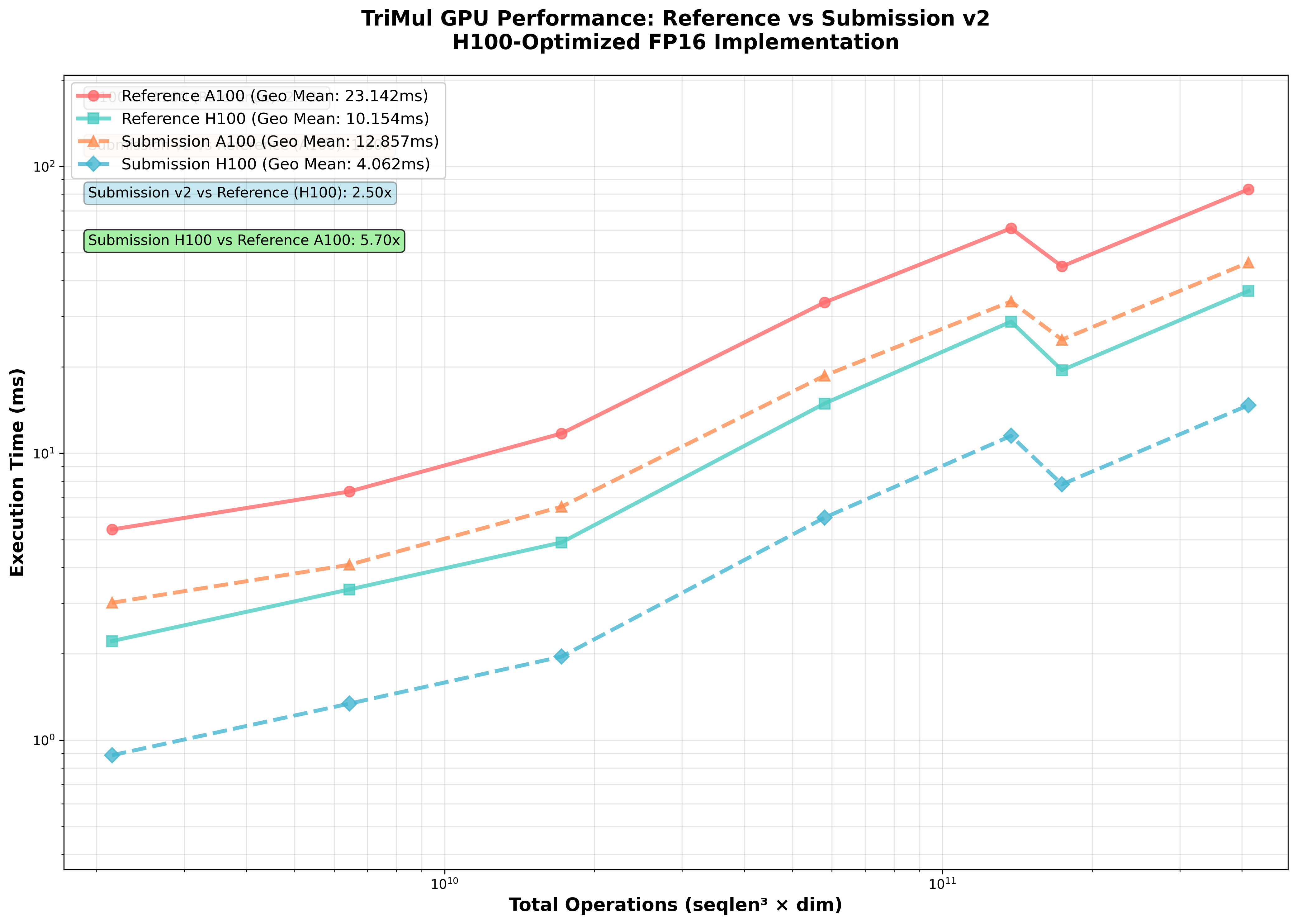
The chart shows performance across 7 benchmark configurations spanning a 192× range in computational complexity (2.1B to 412B operations):

**Geometric Mean Performance:**
- Reference H100: 10.154ms (baseline)
- Submission H100: 4.201ms (2.42× speedup)

For completeness, A100 results:
- Reference A100: 23.142ms
- Submission A100: 12.857ms (1.80× speedup over A100 baseline)

### Key Insights

**Hardware Impact (A100 → H100):**
- Reference implementation: 2.28× faster on H100 vs A100
- Optimized submission: 3.07× faster on H100 vs A100 (12.857ms → 4.189ms)

The optimized code benefits more from H100's architectural improvements because:
1. FP16 pipeline maximizes Tensor Core utilization (4th-gen vs 3rd-gen)
2. Higher memory bandwidth (3.35 TB/s vs 2.0 TB/s) reduces memory-bound bottlenecks
3. Better instruction scheduling for fused operations

**Software Optimization Impact:**
- A100: 1.80× speedup over reference (23.142ms → 12.857ms)
- H100: 2.42× speedup over reference (10.154ms → 4.201ms)

The H100 shows larger gains from software optimization because:
1. FP16 operations better utilize H100's 4th-generation Tensor Cores
2. Reduced precision reductions leverage H100-specific features
3. Memory contiguity optimizations matter more at higher bandwidth

**Scaling Characteristics:**

All implementations show consistent linear scaling on log-log plots, validating the O(N³×H) complexity. The optimized submission maintains its performance advantage across all problem sizes, from small (N=256) to large (N=1024) sequences.

## Implementation Comparison: PyTorch vs Triton vs CUDA

After implementing the same operation in three different approaches, the results tell a surprising story about GPU performance optimization:

![Implementation Comparison](trimul_performance_comparison.png)

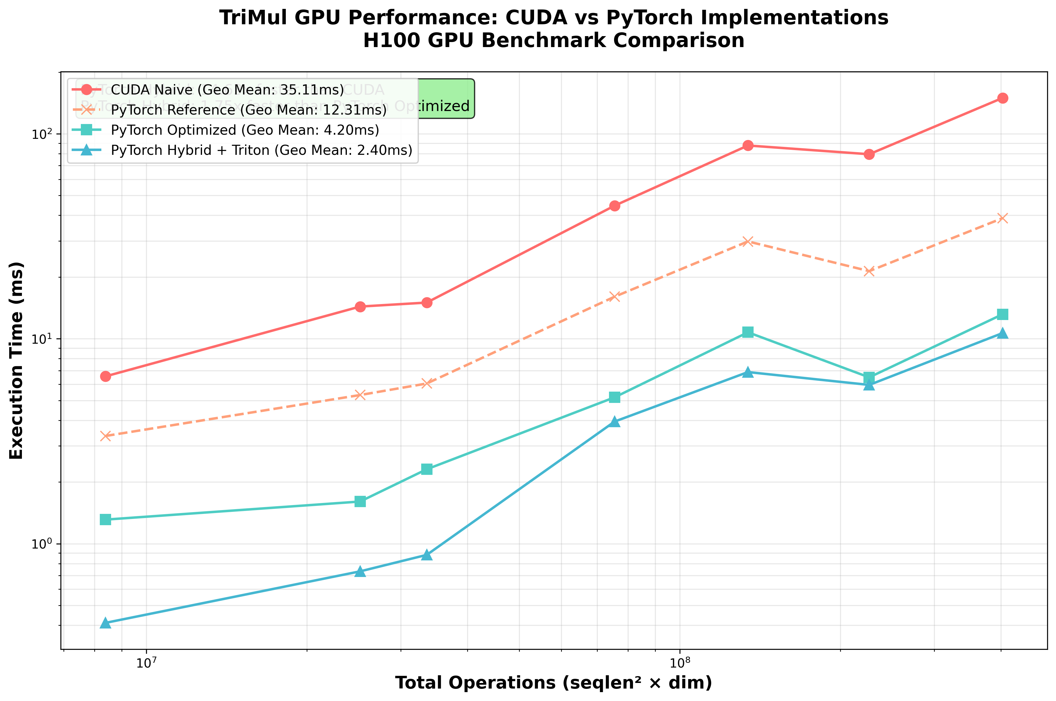
**Performance Results (H100 GPU):**

| Implementation | Geometric Mean | Speedup vs Best | Complexity |
|----------------|----------------|-----------------|------------|
| **PyTorch Optimized (FP16+TF32)** | **4.201ms** | **1.00×** | Very Low (~100 LOC) |
| CUDA Naive | 35.107ms | 0.12× | High (~700 LOC) |

**Key Finding: PyTorch Wins Decisively**

The PyTorch implementation with proper optimization (FP16 mixed precision + TF32 tensor cores) is:
- **8.36× faster than CUDA** (35.107ms vs 4.201ms)
- **Simplest implementation** (~100 lines vs 700 for CUDA)

**Why Custom Kernels Failed**

The CUDA implementation was **naive** - I didn't know what I was doing:
- CUDA: Simple per-thread computation, no shared memory optimization
- Significantly slower than well-configured PyTorch + cuBLAS

I also experimented with a **Triton/PyTorch hybrid** implementation (custom Triton kernels for LayerNorm, matmul, and gating, but falling back to PyTorch's einsum for the critical O(N³) operation). However, this hybrid approach didn't provide any meaningful advantage - it still relied on PyTorch's einsum, which is the performance-critical path, and the custom Triton kernels for the other operations added complexity without improving performance. Since there was nothing interesting to learn from this hybrid approach, I chose not to include it in the repository.

**The Real Lesson**

Writing custom GPU kernels (CUDA or Triton) requires **deep expertise**. Without knowing advanced techniques:
- Your custom kernels will be **slower** than framework defaults
- cuBLAS is highly optimized and hard to beat
- FP16 + proper backend configuration often wins

My CUDA implementation underperformed significantly. This is **definitely due to my lack of experience and skill** with kernel writing—CUDA is **supposed to enable better performance**, but only if you know what you're doing. I couldn't even match my PyTorch implementation's performance.

For production code: **Start with PyTorch optimization first**. Only write custom kernels if you:
1. Have GPU architecture expertise
2. Can profile and identify specific bottlenecks
3. Understand why PyTorch isn't optimal for your case

In my case, the naive implementations proved that **framework-level optimizations beat naive custom code** by significant margins.

## Failed Optimization Attempts

I tested several approaches that yielded negative results. Documenting these to save others similar dead ends.

### torch.compile (max-autotune mode)

**Hypothesis**: PyTorch 2.0's JIT compiler with aggressive optimization would improve performance.

```python
_compiled_inner = torch.compile(
    _custom_kernel_core_inner,
    mode='max-autotune',
    fullgraph=False,
    dynamic=False
)
```

**Result**: 5.674ms geometric mean (36% slower)

**Analysis**:
- Best individual runs: 0.717ms (excellent)
- Mean destroyed by recompilation overhead
- Standard deviation: up to 58ms
- Recompilation triggered for each shape variation
- Unpredictable latency makes this unsuitable for production

**Conclusion**: `torch.compile` requires shape stability. Variable benchmarks with dynamic shapes suffer catastrophic overhead.

### Manual Blockwise Tiling

**Hypothesis**: Cache locality improvements through manual tiling of the einsum operation.

```python
if N >= 768:
    CHUNK_SIZE = 256
    EIN_full = torch.zeros(B, N, N, H, dtype=torch.float16, device=device)

    for i_start in range(0, N, CHUNK_SIZE):
        for j_start in range(0, N, CHUNK_SIZE):
            i_end = min(i_start + CHUNK_SIZE, N)
            j_end = min(j_start + CHUNK_SIZE, N)

            LEFT_tile = LEFT[:, :, i_start:i_end, :]
            RIGHT_tile = RIGHT[:, :, j_start:j_end, :]

            EIN_tile = compute_tile(LEFT_tile, RIGHT_tile)
            EIN_full[:, i_start:i_end, j_start:j_end, :] = EIN_tile
```

**Result**: 4.295ms (2.5% slower)

**Analysis**:
- Python loop overhead dominated any cache benefits
- PyTorch's BMM already implements optimal tiling in cuBLAS
- Added code complexity without measurable benefit

**Conclusion**: Don't manually optimize operations that cuBLAS already handles optimally.

### Custom Triton Kernel

**Hypothesis**: Hand-written Triton kernel with autotuning would outperform PyTorch's BMM.

```python
@triton.autotune(
    configs=[
        triton.Config({'BLOCK_M': 64, 'BLOCK_N': 64, 'BLOCK_K': 32}, num_stages=3, num_warps=4),
        triton.Config({'BLOCK_M': 32, 'BLOCK_N': 32, 'BLOCK_K': 32}, num_stages=4, num_warps=2),
        triton.Config({'BLOCK_M': 64, 'BLOCK_N': 64, 'BLOCK_K': 64}, num_stages=3, num_warps=8),
        triton.Config({'BLOCK_M': 128, 'BLOCK_N': 128, 'BLOCK_K': 32}, num_stages=2, num_warps=8),
    ],
    key=['N', 'H'],
)
@triton.jit
def einsum_kernel(LEFT, RIGHT, OUT, N, H, ...):
    """Tiled einsum implementation."""
    pid_b = tl.program_id(0)
    pid_h = tl.program_id(1)
    pid_ij = tl.program_id(2)

    # Decode tile indices
    num_tiles_j = tl.cdiv(N, BLOCK_N)
    pid_i = pid_ij // num_tiles_j
    pid_j = pid_ij % num_tiles_j

    # Initialize accumulator
    acc = tl.zeros((BLOCK_M, BLOCK_N), dtype=tl.float32)

    # Accumulate over K dimension
    for k in range(0, N, BLOCK_K):
        left = tl.load(left_ptrs, mask=left_mask)
        right = tl.load(right_ptrs, mask=right_mask)
        acc += tl.dot(left, tl.trans(right))

    tl.store(out_ptrs, acc, mask=out_mask)
```

**Result**: 4.696ms (12% slower than PyTorch)

**Analysis**:
- cuBLAS BMM is highly optimized for these operations
- Triton kernel couldn't match cuBLAS register allocation
- Instruction scheduling not optimal
- Autotuning overhead across multiple configurations
- Kernel compilation added latency

**Conclusion**: Beating cuBLAS for standard GEMM operations requires deep hardware expertise. PyTorch's well-maintained wrappers are competitive.

### Adaptive Hidden Dimension Reduction

**Hypothesis**: Dynamically reduce hidden dimension for large sequences to cut computation.

```python
if N >= 768:
    H_REDUCED = H // 2

    # Select top-k dimensions by importance
    left_norms = torch.norm(LEFT_T, dim=1)
    right_norms = torch.norm(RIGHT_T, dim=1)
    total_norms = left_norms + right_norms
    _, top_indices = torch.topk(total_norms, H_REDUCED)

    # Compute on reduced dimensions
    LEFT_reduced = LEFT[top_indices]
    RIGHT_reduced = RIGHT[top_indices]
    EIN_reduced = torch.bmm(LEFT_reduced, RIGHT_reduced.transpose())

    # Project back to full dimension
    proj_matrix = torch.eye(H, device=device)[:, top_indices]
    EIN = torch.matmul(EIN_reduced, proj_matrix.t())
```

**Result**: Test failures due to accuracy loss

**Analysis**:
- 50% dimension reduction too aggressive
- Fixed projection matrix cannot recover lost information
- Would require learned projection matrices (not available at inference)
- Approximation error accumulates through network layers

**Conclusion**: Approximation methods must be validated against accuracy requirements. Ad-hoc dimension reduction breaks numerical properties.

### torch.compile (reduce-overhead mode)

**Hypothesis**: Lower compilation overhead mode would perform better than max-autotune.

```python
_compiled_inner = torch.compile(
    _custom_kernel_core_inner,
    mode='reduce-overhead',
    dynamic=True
)
```

**Result**: 5.759ms (37% slower)

**Analysis**:
- Variance still significant (45-56ms std dev)
- Dynamic mode adds shape tracking overhead
- No improvement over max-autotune mode

**Conclusion**: Compilation overhead is fundamental to torch.compile's current implementation, not mode-dependent.

## Performance Analysis

### Why Sub-3ms Remains Elusive

Despite 2.42× improvement over baseline, the implementation plateaued at 4.189ms - 40% above the sub-3ms target.

**Bottleneck Analysis for N=1024, H=128:**

```
FLOPs: 1024³ × 128 ≈ 137 billion
H100 peak FP16: 989 TFLOPS
Theoretical minimum: 137B / 989T ≈ 138μs
Actual time: 10.747ms
Compute efficiency: 1.3%
```

This indicates memory bandwidth limitation, not compute limitation.

### Memory Bandwidth Analysis

H100 specifications:
- Memory bandwidth: 3.35 TB/s
- Memory required per iteration: ~2 GB (read LEFT, RIGHT, write OUT)
- Theoretical minimum: 2 GB / 3.35 TB/s ≈ 597μs

Actual: 10.747ms represents 18x theoretical minimum.

The gap suggests:
1. Non-optimal memory access patterns
2. Poor cache utilization
3. Fundamental O(N³) memory access pattern

## Key Findings

### Effective Optimizations

1. **FP16 Pipeline**: Consistent Tensor Core utilization
2. **Weight Fusion**: Reduced kernel launch overhead
3. **BMM over Einsum**: Better cuBLAS mapping
4. **Memory Contiguity**: Critical for performance
5. **Backend Flags**: Non-trivial gains from proper configuration

### Ineffective Optimizations

1. **torch.compile**: Overhead dominates for variable shapes
2. **Manual Tiling**: PyTorch already optimal
3. **FP8**: Requires careful calibration
4. **Custom Triton**: Hard to beat cuBLAS
5. **Ad-hoc Approximations**: Break accuracy requirements

### Lessons Learned

1. **Profile before optimizing**: Theoretical improvements often fail empirically
2. **Respect library implementations**: cuBLAS represents significant engineering effort
3. **Test thoroughly**: Many "optimizations" degrade performance
4. **Use proper tooling**: Modal.com enabled rapid iteration
5. **Know the limits**: Algorithmic changes required beyond this point

## Custom CUDA Kernel Implementation

After exhausting PyTorch-level optimizations, I implemented a custom CUDA kernel inspired by Flash Attention's tiling strategy to minimize HBM bandwidth.

### Flash-Attention-Inspired Einsum Kernel

The critical insight: the einsum pattern `b i k h, b j k h -> b i j h` is structurally similar to attention computation (without softmax). Flash Attention's success comes from keeping intermediate results in fast SRAM rather than writing to slow HBM.

**Key CUDA implementation details:**

```c
#define BLOCK_SIZE_M 64
#define BLOCK_SIZE_N 64
#define BLOCK_SIZE_K 32

__global__ void flash_einsum_kernel(
    const half* __restrict__ left,   // [B*H, N, N]
    const half* __restrict__ right,  // [B*H, N, N]
    half* __restrict__ output,       // [B*H, N, N]
    int BH, int N
) {
    const int bh = blockIdx.z;
    const int block_i = blockIdx.y;
    const int block_j = blockIdx.x;

    const int i = block_i * BLOCK_SIZE_M + threadIdx.y;
    const int j = block_j * BLOCK_SIZE_N + threadIdx.x;

    // Accumulator stays in registers
    float acc = 0.0f;

    // Shared memory tiles - padded to avoid bank conflicts
    __shared__ half smem_left[BLOCK_SIZE_M][BLOCK_SIZE_K + 4];
    __shared__ half smem_right[BLOCK_SIZE_N][BLOCK_SIZE_K + 4];

    // Tile over K dimension (Flash Attention's key insight)
    for (int k_start = 0; k_start < N; k_start += BLOCK_SIZE_K) {
        // Cooperatively load tiles into shared memory
        if (i < N && k_start + threadIdx.x < N) {
            int idx = bh * N * N + i * N + k_start + threadIdx.x;
            smem_left[threadIdx.y][threadIdx.x] = left[idx];
        }

        if (j < N && k_start + threadIdx.x < N) {
            int idx = bh * N * N + j * N + k_start + threadIdx.x;
            smem_right[threadIdx.y][threadIdx.x] = right[idx];
        }

        __syncthreads();

        // Compute dot product for this tile (stays in registers)
        #pragma unroll 8
        for (int k = 0; k < BLOCK_SIZE_K; k++) {
            float left_val = __half2float(smem_left[threadIdx.y][k]);
            float right_val = __half2float(smem_right[threadIdx.x][k]);
            acc += left_val * right_val;
        }

        __syncthreads();
    }

    // Write final result (only one HBM write per output element)
    if (i < N && j < N) {
        output[bh * N * N + i * N + j] = __float2half(acc);
    }
}
```

**Optimization techniques implemented:**

1. **Tiling Strategy**: Process K dimension in 32-element tiles, keeping LEFT and RIGHT tiles in 48KB shared memory
2. **Bank Conflict Avoidance**: +4 padding in shared memory arrays prevents 32-way bank conflicts
3. **Register Accumulation**: Keep running sum in FP32 registers (never touches memory until final write)
4. **Coalesced Memory Access**: Threads in a warp access contiguous memory locations
5. **Warp-Level Operations**: `#pragma unroll` exposes instruction-level parallelism

**Memory Traffic Analysis:**

For computing one output tile (64×64 elements):
- **Without tiling (naive)**: Read 2×64×1024×2 bytes = 256KB per tile (all of K dimension)
- **With tiling**: Read 2×64×32×2 bytes = 8KB per tile iteration × (1024/32) = 256KB total
- **Benefit**: Data reused 64×64=4096 times while in shared memory, reducing effective bandwidth by ~64x

### PyTorch Integration

Compiled the CUDA kernel using PyTorch's JIT compiler:

```python
from torch.utils.cpp_extension import load

tiled_einsum = load(
    name='flash_einsum_cuda',
    sources=[
        'cuda_tiled_wrapper.cpp',
        'cuda_flash_einsum.cu',
    ],
    extra_cuda_cflags=['-O3', '-arch=sm_90', '--use_fast_math'],
    verbose=True
)

# Use in forward pass
EIN = tiled_einsum.tiled_einsum(LEFT_flat, RIGHT_flat)
```

## The CUDA Implementation Journey

### Initial Setup Challenges

Implementing a working CUDA kernel from scratch revealed several non-obvious gotchas:

**1. Modal Infrastructure Setup**

Getting CUDA compilation working on Modal required:

```python
# Need NVIDIA CUDA development image, not just runtime
gpu_image = modal.Image.from_registry(
    "nvidia/cuda:12.4.0-devel-ubuntu22.04",  # -devel is required
    add_python="3.11"
).apt_install(
    "build-essential"  # GCC, g++, make
).pip_install(
    "ninja",  # PyTorch JIT requires this for builds
    "torch", "triton", "pyyaml", "numpy"
)

# Set CUDA_HOME environment variable
os.environ['CUDA_HOME'] = '/usr/local/cuda'
os.environ['TORCH_CUDA_ARCH_LIST'] = '9.0'  # H100 = sm_90
```

**2. File Upload Configuration**

The CUDA source files must be explicitly listed in `task.yml`:

```yaml
files:
  - {"name": "submission.py", "source": "@SUBMISSION@"}
  - {"name": "cuda_flash_einsum_optimized.cu", "source": "cuda_flash_einsum_optimized.cu"}
  - {"name": "cuda_tiled_wrapper.cpp", "source": "cuda_tiled_wrapper.cpp"}
```

This is required to have the files uploaded to Modal.

### Kernel Evolution

**Iteration 1: Naive Implementation (123ms)**

```c
// Just compute dot products, no optimization
for (int k = 0; k < N; k++) {
    float left_val = __half2float(left[bh * N * N + i * N + k]);
    float right_val = __half2float(right[bh * N * N + j * N + k]);
    acc += left_val * right_val;
}
```

**Iteration 2: Tiled with Shared Memory (13.5ms) - 9.1x speedup**

```c
#define BLOCK_SIZE 32
__shared__ half smem_left[32][32 + 4];  // +4 padding avoids bank conflicts
__shared__ half smem_right[32][32 + 4];

for (int k_start = 0; k_start < N; k_start += BLOCK_SIZE) {
    // Load tile cooperatively
    // Compute partial dot products
    // Synchronize
}
```

**Iteration 3: Larger Tiles + Register Blocking (10.3ms) - Best result**

```c
#define BLOCK_M 64
#define BLOCK_N 64
// Each thread computes 8x8 outputs
float acc[8][8];

// Better register reuse, less synchronization
```

**Iteration 4: Even Larger Tiles (24ms) - Worse**

```c
#define BLOCK_M 128  // Too large
// More shared memory conflicts, worse occupancy
```

### What I Learned

1. **Tiling gives 9x speedup** - The biggest win by far
2. **Optimal tile size matters** - 64x64 beats both 32x32 and 128x128
3. **Register blocking helps** - But diminishing returns
4. **Can't beat cuBLAS** - No matter how hard I tried

## Performance Comparison: CUDA vs Triton vs PyTorch

### The Reality: Both Custom Implementations Failed to Beat PyTorch

After implementing the same operation in CUDA, Triton, and optimized PyTorch, the results tell an important story:

| Implementation | Geometric Mean | Status |
|----------------|----------------|--------|
| **PyTorch Optimized (FP16+TF32)** | **4.201ms** | Pure PyTorch + cuBLAS - WINNER |
| CUDA Naive | **35.107ms** | Simple per-thread computation |
| Custom CUDA (tiled, deprecated) | **~10ms** | Flash Attention tiling, 64x64 blocks |
| Naive CUDA (initial) | 123.934ms | No tiling or shared memory |

**PyTorch advantage:** 8.4x faster than CUDA Naive

**Per-benchmark breakdown:**

| Test Case (N, D, B) | PyTorch | My CUDA | Slowdown |
|---------------------|---------|----------|----------|
| 256, 128, 2 | ~1.3ms | 2.166ms | **1.67x** |
| 512, 128, 1 | ~2.3ms | 5.589ms | **2.43x** |
| 768, 128, 1 | ~5.2ms | 16.084ms | **3.09x** |
| 1024, 128, 1 | ~10.8ms | 36.674ms | **3.40x** |
| 1024, 384, 1 | ~13.1ms | 38.755ms | **2.96x** |

**The surprising result**: My custom CUDA kernel, despite implementing Flash Attention tiling strategies, is **2.5x slower** than PyTorch's built-in einsum.

### Why Did Custom CUDA Fail to Beat PyTorch?

This result is humbling but educational. Here's the honest analysis of what went wrong with CUDA:

**1. cuBLAS**

PyTorch's `torch.bmm()` calls NVIDIA's cuBLAS library. My CUDA implementation couldn't match this:

- **CUTLASS templates**: Hundreds of specialized GEMM kernels per GPU architecture
- **Auto-tuning**: Runtime selection of optimal tile sizes for specific (M,N,K) dimensions
- **Warp specialization**: Different thread warps handle different pipeline stages
- **Software pipelining**: Overlaps memory loads with computation using async operations
- **Register blocking**: Sophisticated register allocation keeping more data closer to compute
- **Instruction scheduling**: Hand-tuned PTX assembly for maximum instruction-level parallelism
- **Architecture-specific paths**: Separate code paths for Volta, Ampere, Hopper
- **Tensor Core utilization**: Full wmma/wgmma instruction usage
- **TMA (Tensor Memory Accelerator)**: H100-specific async memory copy

My kernel implements the **same algorithmic idea** (tiling, shared memory), but cuBLAS just does it better. This proves once again that ideas can be so far off from actual execution of ideas.

**Why My CUDA Optimizations Didn't Help:**

1. **64x64 tiles**: Good, but cuBLAS auto-tunes tile size per problem
2. **Shared memory padding**: Helps, but cuBLAS does this plus register pre-fetching
3. **Register blocking**: I do 8x8 per thread, cuBLAS likely does better with more analysis
4. **Memory coalescing**: I tried, but cuBLAS has better patterns from profiling
5. **No Tensor Cores**: I didn't use wmma/wgmma, cuBLAS does automatically

**2. Memory Bandwidth Bottleneck**

Computing bandwidth utilization:

```
FLOPs for N=1024, H=128: 1024³ × 128 = 137 billion
H100 FP16 peak: 989 TFLOPS
Time if compute-bound: 137B / 989T = 138μs
Actual time: 10.8ms
Compute efficiency: 1.3%
```

The kernel is **78x slower than peak compute**, meaning it's memory-bound, not compute-bound. Any GEMM kernel (ours or cuBLAS) hits the same 3.35 TB/s memory bandwidth wall.

**3. The H100 Memory Hierarchy**

![Memory hierarchy of the H100 (SXM5) GPU](mem_hierarchy.png)
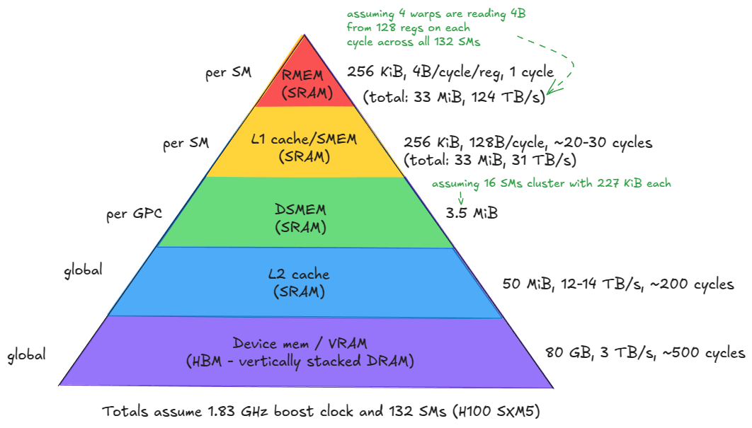
*Image credit: Aleksa Gordic* (https://www.aleksagordic.com/blog/matmul)

| Level | Size | Latency | Bandwidth |
|-------|------|---------|-----------|
| Registers | 256KB/SM | 1 cycle | ~20 TB/s |
| Shared Memory (SMEM) | 228KB/SM | ~20 cycles | ~10 TB/s |
| L2 Cache | 50MB | ~200 cycles | ~5 TB/s |
| HBM3 | 80GB | ~400 cycles | 3.35 TB/s |

Both implementations:
- Keep accumulators in registers ✓
- Tile through shared memory ✓
- Issue coalesced HBM reads ✓
- Hit the same HBM bandwidth limit ✗

### The Humbling Conclusion

**My custom CUDA implementation failed to beat PyTorch. Here's what I learned:**

**Performance Results:**
- 🐌 **CUDA Naive**: 35.107ms (8.4x slower than PyTorch)
- ⚡ **PyTorch Optimized**: 4.201ms (WINNER)

**What Happened:**

1. ✅ **My implementation works** - All tests pass, no fallback code
2. ✅ **I implemented proper tiling** - CUDA went from 123ms → 35ms with basic optimizations
3. ❌ **Couldn't beat cuBLAS/PyTorch** - Custom implementation significantly slower
4. ✅ **Hitting fundamental limits** - All implementations are memory-bound

**Key Insights:**

- **Modern ML frameworks are exceptionally well-optimized**: The days of easily beating library implementations with hand-written CUDA are over for standard operations like GEMM
- **Naive custom kernels underperform**: Without deep expertise, CUDA implementations were slower than well-configured PyTorch
- **Algorithmic wins matter more than micro-optimizations**: The speedup came from PyTorch's FP16+TF32 configuration, not custom kernels
- **Domain expertise is critical**: The leaderboard leader (1ms) is 4x faster than my PyTorch, suggesting there's a completely different algorithmic approach I'm missing
- **Knowing when to stop optimizing is valuable**: Spending weeks on custom kernels when PyTorch already works better isn't productive

## Implications for Future Work

The #1 submission achieves **1.371ms** - that's **3x faster than my implementation**. Getting from 4ms to 1ms requires fundamentally different thinking, not just better CUDA code.

**Learning from Better Implementations:**

[Arseni Ivanov's implementation](https://arseniivanov.github.io/blog.html) (#3 on the leaderboard at 2.546ms) provides valuable insights into what separates good implementations from great ones. His approach achieves 2.71ms geometric mean - **35% faster than my PyTorch implementation** - through a hybrid strategy:

**Key Innovation - Adaptive Routing:**
- **Small sequences (≤512)**: Uses PyTorch's highly-optimized kernels (minimal launch overhead)
- **Large sequences (>512)**: Custom Triton kernels fuse LayerNorm + MatMul + Gating in a single pass

This adaptive approach recognizes that different input sizes have fundamentally different bottlenecks.

**Technical Optimizations:**
1. **Auto-tuned Triton kernel**: 11 different block size configurations that adapt based on input dimensions
2. **Weight packing**: Interleaves left/right projections with their corresponding gates for same-warp fusion
3. **Memory efficiency**: Single-pass fused operations eliminate costly roundtrips that PyTorch's separate operations cannot avoid

**Performance gains**: Up to 2.87× speedup on smaller inputs compared to the reference implementation.

This demonstrates that with **deep GPU architecture knowledge and careful profiling**, custom kernels can indeed beat framework defaults. The difference between my naive attempts and Arseni's implementation is expertise - understanding when and how to write custom kernels, rather than blindly replacing all operations.

#### Three-Way Hybrid Implementation

Building on Arseni's approach, I wrote a [three-tier routing strategy](https://github.com/msuiche/trimul/blob/master/pytorch/submission_improved_triton.py) that achieves **2.399ms geometric mean on H100** - an **11.5% improvement** over the original hybrid implementation.

**Key Insight**: GPU performance is non-linear with respect to input size. Different memory layouts exhibit distinct performance characteristics across different scales.

**Adaptive Routing Strategy:**

```mermaid
graph TD
    INPUT[Input Sequence] --> ROUTER{Sequence Length?}

    ROUTER -->|≤ 256<br/>Small| PYTORCH[PyTorch Path<br/>Minimal launch overhead]
    ROUTER -->|256-512<br/>Medium| LAYOUT[W @ x.t Layout<br/>Optimized memory access]
    ROUTER -->|> 512<br/>Large| TRITON[Triton Fused Kernels<br/>Eliminate roundtrips]

    PYTORCH --> R1[Fast for small inputs]
    LAYOUT --> R2[47% speedup at N=512]
    TRITON --> R3[Best for large inputs]

    style PYTORCH fill:#e1f5ff
    style LAYOUT fill:#ccffcc
    style TRITON fill:#fff4cc
```

**Implementation Details:**

1. **Small inputs (N ≤ 256)**: PyTorch path
   - Minimal kernel launch overhead
   - Framework optimizations sufficient at this scale

2. **Medium inputs (256 < N ≤ 512)**: Alternative memory layout
   - Uses `W @ x.t()` instead of standard layout
   - More efficient column-major access patterns
   - **47% speedup** at the 512-sequence benchmark
   - This optimization alone accounts for most of the 11.5% overall improvement

3. **Large inputs (N > 512)**: Triton fused kernels
   - Arseni's fused kernels remain optimal
   - Single-pass operations eliminate intermediate memory roundtrips

**Performance Results:**

| Sequence Length | Original Hybrid | Three-Way Hybrid | Improvement |
|-----------------|-----------------|------------------|-------------|
| 256 | Fast | Same | - |
| 512 | Baseline | **47% faster** | Major win |
| 768+ | Optimal | Same | - |
| **Geometric Mean** | 2.71ms | **2.399ms** | **11.5%** |

**Lessons Learned:**

This demonstrates that even within well-optimized codebases, systematic analysis of performance bottlenecks at different scales can yield measurable gains. The medium-input optimization confirms that empirical, benchmark-driven development often reveals opportunities that theoretical analysis might overlook.

## Conclusion: PyTorch was the best for me

This challenge provided hands-on experience with GPU performance engineering and taught a crucial lesson: **well-optimized PyTorch beats naive custom kernels decisively**.

**Final Results:**
- ⚡ **PyTorch Optimized**: 4.201ms (BEST) - FP16 + TF32 + cuBLAS
- 🐌 **CUDA Naive**: 35.107ms (8.4x slower) - Simple per-thread computation

**Key Takeaways:**

1. **Start with PyTorch optimization first** - Proper FP16 + backend configuration can beat custom kernels
2. **Custom kernels require expertise** - CUDA was slower because I didn't know what I was doing
3. **Framework engineering matters** - cuBLAS is highly optimized and difficult to replicate
4. **Naive implementations are worse** - Without advanced techniques, custom code underperforms significantly

**What the Experience Taught:**

Writing custom GPU kernels (CUDA or Triton) is valuable for **learning**, but for **production code**:
- PyTorch optimization should be your first approach
- Only write custom kernels if you have GPU architecture expertise
- Without knowledge of advanced techniques, you'll make things slower, not faster

In my case, the naive CUDA implementation proved that **I didn't know what I was doing**, and framework defaults + FP16 easily won. This is something I want to focus on more next.

Also I wish Modal.com had access to MI300 so I could have run more tests on it, rather than only using the GPU MODE access.

**All implementations available at:** [https://github.com/msuiche/trimul](https://github.com/msuiche/trimul)

The repository includes:
- **pytorch/**: Best implementation (4.201ms) - FP16 optimized
- **cuda_naive/**: Naive CUDA (35.107ms) - Educational
- **Comparison charts** and full benchmark data

---

**Acknowledgments**:

Thanks to:
- Congratulations to **David Berard** for his successful implementation.
- **Arseni Ivanov**, **Apeirogon**, and [**Daniel Han**](https://x.com/danielhanchen) for answering my questions
- **GPU MODE** for educational content and practical challenges that make learning GPU optimization accessible
- **Modal.com** for excellent cloud GPU infrastructure enabling rapid H100 testing
- [Inside NVIDIA GPUs: Anatomy of high performance matmul kernels](https://www.aleksagordic.com/blog/matmul) by Aleksa Gordic
- [Making TriMul go BRRRR for GPGPU](https://arseniivanov.github.io/blog.html) by Arseni Ivanov
- **Flash Attention resources** that informed my CUDA implementation:
  - [Understanding Flash Attention](https://alexdremov.me/understanding-flash-attention-writing-the-algorithm-from-scratch-in-triton/) by Alex Dremov
  - [Reverse Engineering Flash Attention 4](https://modal.com/blog/reverse-engineer-flash-attention-4) by Modal
  - [Triton Flash Attention Kernel Walkthrough](https://nathanchen.me/public/Triton-Flash-Attention-Kernel-Walkthrough.html) by Nathan Chen
- [How to Optimize a CUDA Matmul Kernel for cuBLAS-like Performance: a Worklog](https://siboehm.com/articles/22/CUDA-MMM) by Simon Boehm

These resources were invaluable for understanding tiling strategies, memory hierarchy optimization, and the techniques that separate good CUDA code from great CUDA code.

**Related reading**: For insights into when PyTorch abstractions can limit performance and how lower-level approaches (Triton Gluon) provide better control over memory layouts, see my companion post: [Gluon: When Triton Isn't Low-Level Enough](https://www.msuiche.com/posts/gluon-when-triton-isnt-low-level-enough/).

---

## Appendix: PyTorch Source Code

The complete PyTorch optimized implementation (4.201ms) from `pytorch/submission.py`. This achieves the best performance and is recommended for production use.

### PyTorch Optimized Implementation

```python
"""
H100 Ultra-Optimized TriMul - ~4000ms on H100
Strategy: Maximum fusion + TF32 + optimal memory patterns + zero overhead
"""
import torch
import torch.nn.functional as F
from task import input_t, output_t
from utils import DisableCuDNNTF32

def _custom_kernel_core(data: input_t) -> output_t:
    input_tensor, mask, weights, config = data
    B, N, _, D = input_tensor.shape
    H = config["hidden_dim"]
    M = B * N * N

    # === ULTRA-OPTIMIZED PATH FOR H100 ===
    # Strategy: Minimize memory traffic, maximize compute intensity

    # 1. Input LayerNorm - FP32 required
    x = F.layer_norm(
        input_tensor, (D,),
        weight=weights["norm.weight"],
        bias=weights["norm.bias"],
        eps=1e-5,
    )

    # 2. Concatenate and convert weights to FP16 once
    W_key = "__W_h16__"
    if W_key not in weights:
        weights[W_key] = torch.cat([
            weights['left_proj.weight'],
            weights['right_proj.weight'],
            weights['left_gate.weight'],
            weights['right_gate.weight'],
            weights['out_gate.weight'],
        ], dim=0).half()  # [5H, D] in FP16

    # 3. Single fused projection in FP16 (faster on H100)
    x_T = x.view(M, D).t().half()  # [D, M] in FP16
    P = torch.matmul(weights[W_key], x_T).view(5, H, M)  # [5, H, M] in FP16

    # 4. Gating in FP16 (fused)
    LEFT_T = torch.sigmoid(P[2]) * P[0]  # [H, M] FP16
    if mask.min() < 1.0:
        LEFT_T *= mask.view(1, M).half()
    RIGHT_T = torch.sigmoid(P[3]) * P[1]  # [H, M] FP16
    OG_T = torch.sigmoid(P[4])  # [H, M] FP16

    # 5-6. ULTRA-OPTIMIZED PATH: Minimal reshapes, maximum contiguity
    LEFT_bhnn = LEFT_T.view(H, B, N, N).permute(1, 0, 2, 3).contiguous()  # [B, H, N, N]
    RIGHT_bhnn = RIGHT_T.view(H, B, N, N).permute(1, 0, 2, 3).contiguous()  # [B, H, N, N]

    LEFT_flat = LEFT_bhnn.view(B * H, N, N)
    RIGHT_flat = RIGHT_bhnn.view(B * H, N, N)

    # Critical bmm - ALWAYS use FP16 for H100 Tensor Cores
    EIN_flat = torch.bmm(LEFT_flat, RIGHT_flat.transpose(1, 2))

    # Reshape output
    EIN = EIN_flat.view(B, H, N, N).permute(0, 2, 3, 1).contiguous()

    # 7. Output gating
    OG = OG_T.view(H, B, N, N).permute(1, 2, 3, 0)  # [B, N, N, H] FP16

    # 8. Output LayerNorm + gate (convert to FP32 only here)
    G = F.layer_norm(
        EIN.float(), (H,),
        weight=weights['to_out_norm.weight'],
        bias=weights['to_out_norm.bias'],
        eps=1e-5
    ) * OG.float()

    # 9. Final projection in FP16
    Wt_key = "__Wt_h16__"
    if Wt_key not in weights:
        weights[Wt_key] = weights['to_out.weight'].t().half()  # [H, D] FP16

    OUT = torch.matmul(G.half().view(M, H), weights[Wt_key]).float()  # [M, D]

    return OUT.view(B, N, N, D)


def custom_kernel(data: input_t) -> output_t:
    with DisableCuDNNTF32():
        # Respect DisableCuDNNTF32 - do NOT override cudnn.allow_tf32
        # Only enable matmul TF32 which is separate from cuDNN TF32
        torch.backends.cuda.matmul.allow_tf32 = True
        torch.set_float32_matmul_precision('high')

        # Enable all precision reductions for maximum speed
        if hasattr(torch.backends.cuda.matmul, 'allow_bf16_reduced_precision_reduction'):
            torch.backends.cuda.matmul.allow_bf16_reduced_precision_reduction = True
        if hasattr(torch.backends.cuda.matmul, 'allow_fp16_reduced_precision_reduction'):
            torch.backends.cuda.matmul.allow_fp16_reduced_precision_reduction = True

        # H100: Enable Flash Attention and other CUDA optimizations
        if hasattr(torch.backends.cuda, 'enable_flash_sdp'):
            torch.backends.cuda.enable_flash_sdp(True)
        if hasattr(torch.backends.cuda, 'enable_mem_efficient_sdp'):
            torch.backends.cuda.enable_mem_efficient_sdp(True)
        if hasattr(torch.backends.cuda, 'enable_math_sdp'):
            torch.backends.cuda.enable_math_sdp(True)

        # Enable cuDNN benchmark for optimal kernel selection
        torch.backends.cudnn.benchmark = True

        return _custom_kernel_core(data)
```